library(tidymodels)
library(tidyverse)
library(here)
library(dotwhisker)Flu Data Model Fitting
Modeling!
Load packages
Load data
symptoms_fit <- readRDS(here("fluanalysis/data/processed_data/symptoms_clean.RDS"))
tibble(symptoms_fit) #quick look at data
# A tibble: 730 × 32
SwollenLymph…¹ Chest…² Chill…³ Nasal…⁴ CoughYN Sneeze Fatigue Subje…⁵ Heada…⁶
<fct> <fct> <fct> <fct> <fct> <fct> <fct> <fct> <fct>
1 Yes No No No Yes No Yes Yes Yes
2 Yes Yes No Yes Yes No Yes Yes Yes
3 Yes Yes Yes Yes No Yes Yes Yes Yes
4 Yes Yes Yes Yes Yes Yes Yes Yes Yes
5 Yes No Yes No No No Yes Yes Yes
6 No No Yes No Yes Yes Yes Yes Yes
7 No No Yes No Yes No Yes Yes No
8 No Yes Yes Yes Yes Yes Yes Yes Yes
9 Yes Yes Yes Yes Yes No Yes Yes Yes
10 No Yes No Yes Yes No Yes No Yes
# … with 720 more rows, 23 more variables: Weakness <fct>, WeaknessYN <fct>,
# CoughIntensity <fct>, CoughYN2 <fct>, Myalgia <fct>, MyalgiaYN <fct>,
# RunnyNose <fct>, AbPain <fct>, ChestPain <fct>, Diarrhea <fct>,
# EyePn <fct>, Insomnia <fct>, ItchyEye <fct>, Nausea <fct>, EarPn <fct>,
# Hearing <fct>, Pharyngitis <fct>, Breathless <fct>, ToothPn <fct>,
# Vision <fct>, Vomit <fct>, Wheeze <fct>, BodyTemp <dbl>, and abbreviated
# variable names ¹SwollenLymphNodes, ²ChestCongestion, ³ChillsSweats, …Data looks good to go
Model fitting 1: Predicting body temp using multivariate linear regression
Split data into training set and testing set
data_split <- initial_split(symptoms_fit, prop = 3/4)

train_data <- training(data_split)
test_data <- testing(data_split)
Define model
lm_mod <- linear_reg() #set model type as linear regressionCreate recipe
recipe_bodytemp <- recipe(BodyTemp ~ ., data = train_data)Add model and recipe together to create workflow
bodytemp_lm_workflow <- workflow() %>%
  add_model(lm_mod) %>%
  add_recipe(recipe_bodytemp)
Model using the workflow created above
bodytemp_fit <- bodytemp_lm_workflow %>%
  fit(data = train_data)
tidy(bodytemp_fit)
# A tibble: 38 × 5
term estimate std.error statistic p.value
<chr> <dbl> <dbl> <dbl> <dbl>
1 (Intercept) 98.2 0.346 284. 0
2 SwollenLymphNodesYes -0.108 0.106 -1.01 0.313
3 ChestCongestionYes 0.0478 0.115 0.414 0.679
4 ChillsSweatsYes 0.313 0.145 2.15 0.0320
5 NasalCongestionYes -0.213 0.131 -1.63 0.105
6 CoughYNYes 0.405 0.289 1.40 0.163
7 SneezeYes -0.374 0.112 -3.34 0.000912
8 FatigueYes 0.111 0.186 0.596 0.552
9 SubjectiveFeverYes 0.348 0.121 2.88 0.00412
10 HeadacheYes 0.0126 0.149 0.0847 0.933
# … with 28 more rowsCreate a dotwhisker plot to look at regression coefficients
tidy(bodytemp_fit) %>%
  dwplot(dot_args = list(size = 2, color = "black"),
         whisker_args = list(color = "black"),
         vline = geom_vline(xintercept = 0,
                            colour = "grey50", linetype = 2))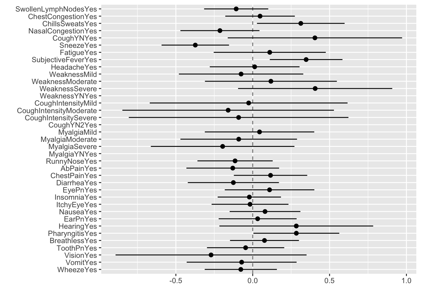
Use model on test data to predict body temp outcome
bodytemp_aug_test <- augment(bodytemp_fit, test_data)Warning in predict.lm(object = object$fit, newdata = new_data, type =
"response"): prediction from a rank-deficient fit may be misleadingbodytemp_aug_test %>% select(BodyTemp, .pred)# A tibble: 183 × 2
BodyTemp .pred
<dbl> <dbl>
1 98.3 99.1
2 100. 99.5
3 102. 99.5
4 98.4 98.8
5 98.2 99.2
6 99.2 98.8
7 98.5 99.0
8 98.2 98.6
9 100. 99.0
10 100 99.0
# … with 173 more rowsUse RMSE to evaluate model
Info on RMSE or Root Mean Squared Error can be found here.
bodytemp_aug_test %>%
  rmse(truth = BodyTemp, .pred)
# A tibble: 1 × 3
.metric .estimator .estimate
<chr> <chr> <dbl>
1 rmse standard 1.20I think this means that this model is estimating body temp incorrectly by this amount (in either direction)
Model fitting 2: Predicting body temp using single-variate linear regression
Predictor of interest: Runny nose
Create recipe
Since we already defined the training set and testing set, we don’t need to do that again. We will just reuse those. We also already defined the model, so we don’t need to do that again.
recipe_bodytemp2 <- recipe(BodyTemp ~ RunnyNose, data = train_data)Here, we have set the outcome of interest to be body temperature, and predictor of interest to be runny nose.
Combine model and recipe to create workflow
bodytemp_lm_workflow2 <- workflow() %>%
  add_model(lm_mod) %>%
  add_recipe(recipe_bodytemp2)
Model using workflow and training data set
bodytemp_fit2 <- bodytemp_lm_workflow2 %>%
  fit(data = train_data)
tidy(bodytemp_fit2)
# A tibble: 2 × 5
term estimate std.error statistic p.value
<chr> <dbl> <dbl> <dbl> <dbl>
1 (Intercept) 99.1 0.0931 1065. 0
2 RunnyNoseYes -0.317 0.110 -2.88 0.00419Now we have trained the model using the training data set.
Create a dotwhisker plot to look at regression coefficient
tidy(bodytemp_fit2) %>%
  dwplot(dot_args = list(size = 2, color = "black"),
         whisker_args = list(color = "black"),
         vline = geom_vline(xintercept = 0,
                            colour = "grey50", linetype = 2))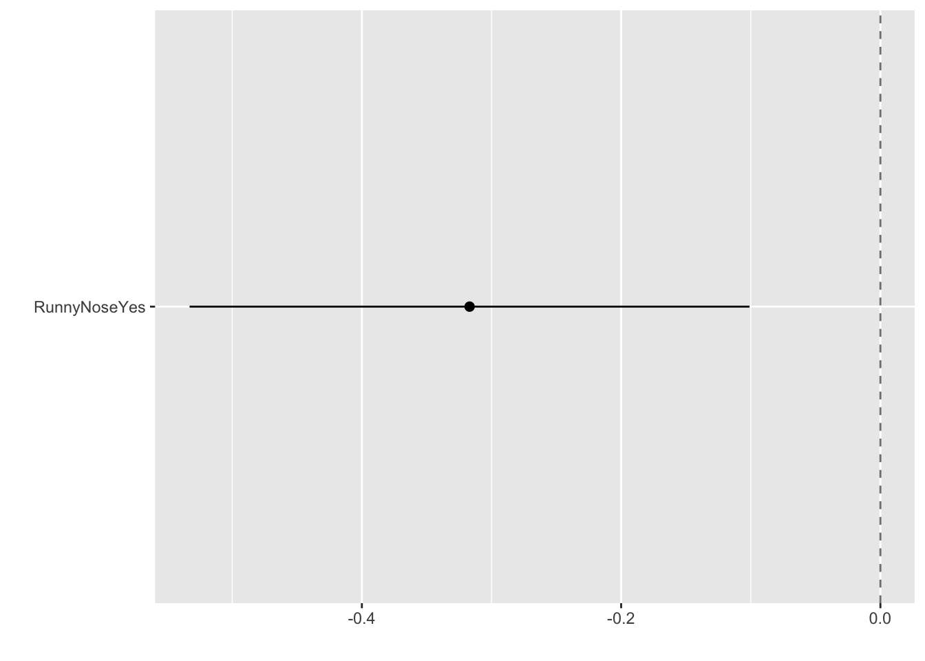
Looks like runny nose is a negative predictor of body temp (body temp is more likely to be lower if runny nose symptom is present)
Use model on test data to predict body temp
bodytemp_aug_test2 <- augment(bodytemp_fit2, test_data)
bodytemp_aug_test2 %>% select(BodyTemp, .pred)
# A tibble: 183 × 2
BodyTemp .pred
<dbl> <dbl>
1 98.3 99.1
2 100. 99.1
3 102. 98.8
4 98.4 98.8
5 98.2 99.1
6 99.2 98.8
7 98.5 98.8
8 98.2 98.8
9 100. 98.8
10 100 98.8
# … with 173 more rowsUse RMSE to evaluate model
bodytemp_aug_test2 %>%
  rmse(truth = BodyTemp, .pred)
# A tibble: 1 × 3
.metric .estimator .estimate
<chr> <chr> <dbl>
1 rmse standard 1.26This is a similar output to what we saw in the first model, where estimation of body temp is slightly off by about 1 degree.
Model fitting 3: Predicting nausea using multivariate logistic regression
Define model
We will continue to use the model testing and training data sets that we created at the start. However, since we now want to create a logistic regression (outcome of interest is categorical), we will need to define a new model
log_mod <- logistic_reg() %>%
  set_engine("glm")
Create recipe
recipe_nausea <- recipe(Nausea ~., data = train_data)This sets the stage to predict nausea outcomes based on all other variables in the data set (predictors)
Combine model and recipe to create workflow
nausea_log_wf <- workflow() %>%
  add_model(log_mod) %>%
  add_recipe(recipe_nausea)
Model using workflow and training data
nausea_fit <- nausea_log_wf %>%
  fit(data = train_data)

nausea_fit %>% extract_fit_parsnip() %>%
  tidy()
# A tibble: 38 × 5
term estimate std.error statistic p.value
<chr> <dbl> <dbl> <dbl> <dbl>
1 (Intercept) -9.21 9.18 -1.00 0.316
2 SwollenLymphNodesYes -0.274 0.231 -1.19 0.235
3 ChestCongestionYes 0.337 0.256 1.32 0.188
4 ChillsSweatsYes 0.254 0.335 0.757 0.449
5 NasalCongestionYes 0.415 0.296 1.40 0.161
6 CoughYNYes -0.382 0.603 -0.633 0.527
7 SneezeYes 0.231 0.245 0.943 0.346
8 FatigueYes 0.0278 0.429 0.0649 0.948
9 SubjectiveFeverYes 0.419 0.267 1.57 0.117
10 HeadacheYes 0.364 0.346 1.05 0.292
# … with 28 more rowsNow we have trained the model, so let’s use the test data to see how well this model predicts nausea.
Use model on test data
predict(nausea_fit, test_data)Warning in predict.lm(object, newdata, se.fit, scale = 1, type = if (type == :
prediction from a rank-deficient fit may be misleading# A tibble: 183 × 1
.pred_class
<fct>
1 No
2 No
3 No
4 No
5 Yes
6 No
7 No
8 No
9 No
10 Yes
# … with 173 more rowsUse ROC curve to assess model fit
Info on ROC curves or Receiver Operating Characteristic can be found here.
nausea_aug_test <- augment(nausea_fit, test_data)

nausea_aug_test %>%
  roc_curve(truth = Nausea, .pred_Yes, event_level = "second") %>%
  autoplot()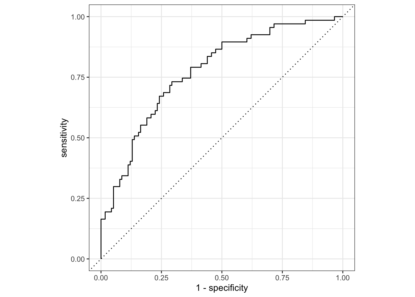
nausea_aug_test %>% roc_auc(truth = Nausea, .pred_Yes,
                            event_level = "second")
# A tibble: 1 × 3
.metric .estimator .estimate
<chr> <chr> <dbl>
1 roc_auc binary 0.773I think what this shows is that the model is a pretty decent predictor of nausea, however, it is more sensitive than it is specific, meaning that it is good at indicating true positives but not as good at indicating true negatives.
Model fitting 4: Predicting nausea using single-variate logistic regression
Predictor of interest: Runny nose
Create recipe
Since we have already split the data and defined the appropriate model, we will just need to create a new recipe that predicts nausea based on runny nose.
recipe_nausea2 <- recipe(Nausea ~ RunnyNose, data = train_data)Combine model and recipe to create workflow
nausea_log_wf2 <- workflow() %>%
  add_model(log_mod) %>%
  add_recipe(recipe_nausea2)
Model using workflow and training data
nausea_fit2 <- nausea_log_wf2 %>%
  fit(data = train_data)

nausea_fit2 %>% extract_fit_parsnip() %>%
  tidy()
# A tibble: 2 × 5
term estimate std.error statistic p.value
<chr> <dbl> <dbl> <dbl> <dbl>
1 (Intercept) -0.590 0.167 -3.54 0.000400
2 RunnyNoseYes -0.0804 0.198 -0.406 0.685 Use model on test data
predict(nausea_fit2, test_data)# A tibble: 183 × 1
.pred_class
<fct>
1 No
2 No
3 No
4 No
5 No
6 No
7 No
8 No
9 No
10 No
# … with 173 more rowsUse ROC curve to assess model fit
nausea_aug_test2 <- augment(nausea_fit2, test_data)

nausea_aug_test2 %>%
  roc_curve(truth = Nausea, .pred_Yes, event_level = "second") %>%
  autoplot()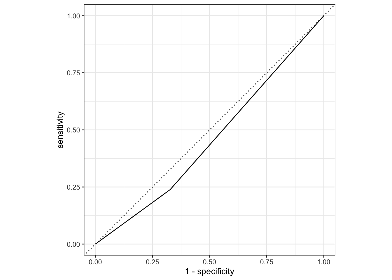
nausea_aug_test2 %>% roc_auc(truth = Nausea, .pred_Yes,
                            event_level = "second")
# A tibble: 1 × 3
.metric .estimator .estimate
<chr> <chr> <dbl>
1 roc_auc binary 0.456