Model Evaluation

Author

Leah Lariscy

Library packages

library(tidymodels)
library(tidyverse)
library(here)
library(dotwhisker)

Load Data

symptoms_fit <- readRDS(here("fluanalysis/data/processed_data/symptoms_clean.RDS"))
colnames(symptoms_fit) #quick look at data

 [1] "SwollenLymphNodes" "ChestCongestion"   "ChillsSweats"     
 [4] "NasalCongestion"   "CoughYN"           "Sneeze"           
 [7] "Fatigue"           "SubjectiveFever"   "Headache"         
[10] "Weakness"          "WeaknessYN"        "CoughIntensity"   
[13] "CoughYN2"          "Myalgia"           "MyalgiaYN"        
[16] "RunnyNose"         "AbPain"            "ChestPain"        
[19] "Diarrhea"          "EyePn"             "Insomnia"         
[22] "ItchyEye"          "Nausea"            "EarPn"            
[25] "Hearing"           "Pharyngitis"       "Breathless"       
[28] "ToothPn"           "Vision"            "Vomit"            
[31] "Wheeze"            "BodyTemp"

Data Split

data_split <- initial_split(symptoms_fit, prop = 3/4) # 75% of data goes into training set

train_data <- training(data_split)
test_data <- testing(data_split)

Model 1 fitting: all variables to predict nausea

Define the model: logistic regression

log_mod <- logistic_reg() %>% #model type is logistic regression 
  set_engine("glm") #engine set to generalized linear model

I am using a logistic regression here because the outcome of interest (Nausea Y/N) is categorical

Create recipe

recipe_nausea <- recipe(Nausea ~., data = train_data)

Nausea is the outcome and all other variables are predictors

Create workflow: combine model definition and recipe

nausea_log_wf <- workflow() %>% 
  add_model(log_mod) %>% #model definition 
  add_recipe(recipe_nausea) #model recipe

This will run a logistic regression on the flu data, predicting nausea using all other variables that we kept.

Model fitting

set.seed(626)
nausea_fit <- nausea_log_wf %>% 
  fit(data = train_data)

nausea_fit %>% extract_fit_parsnip() %>% 
  tidy()

# A tibble: 38 × 5
   term                 estimate std.error statistic p.value
   <chr>                   <dbl>     <dbl>     <dbl>   <dbl>
 1 (Intercept)            0.386      9.31     0.0414  0.967 
 2 SwollenLymphNodesYes  -0.0795     0.230   -0.346   0.729 
 3 ChestCongestionYes     0.110      0.249    0.440   0.660 
 4 ChillsSweatsYes        0.743      0.369    2.02    0.0438
 5 NasalCongestionYes     0.344      0.300    1.14    0.252 
 6 CoughYNYes            -0.206      0.613   -0.336   0.737 
 7 SneezeYes              0.217      0.254    0.855   0.393 
 8 FatigueYes             0.157      0.423    0.371   0.711 
 9 SubjectiveFeverYes    -0.157      0.272   -0.579   0.563 
10 HeadacheYes            0.272      0.333    0.814   0.415 
# … with 28 more rows

Model assessment on training data: ROC curve

set.seed(626)
nausea_aug_test <- augment(nausea_fit, train_data)

nausea_aug_test %>% 
  roc_curve(truth = Nausea, .pred_Yes, event_level = "second") %>% 
  autoplot()

nausea_aug_test %>% roc_auc(truth = Nausea, .pred_Yes, 
                            event_level = "second")

# A tibble: 1 × 3
  .metric .estimator .estimate
  <chr>   <chr>          <dbl>
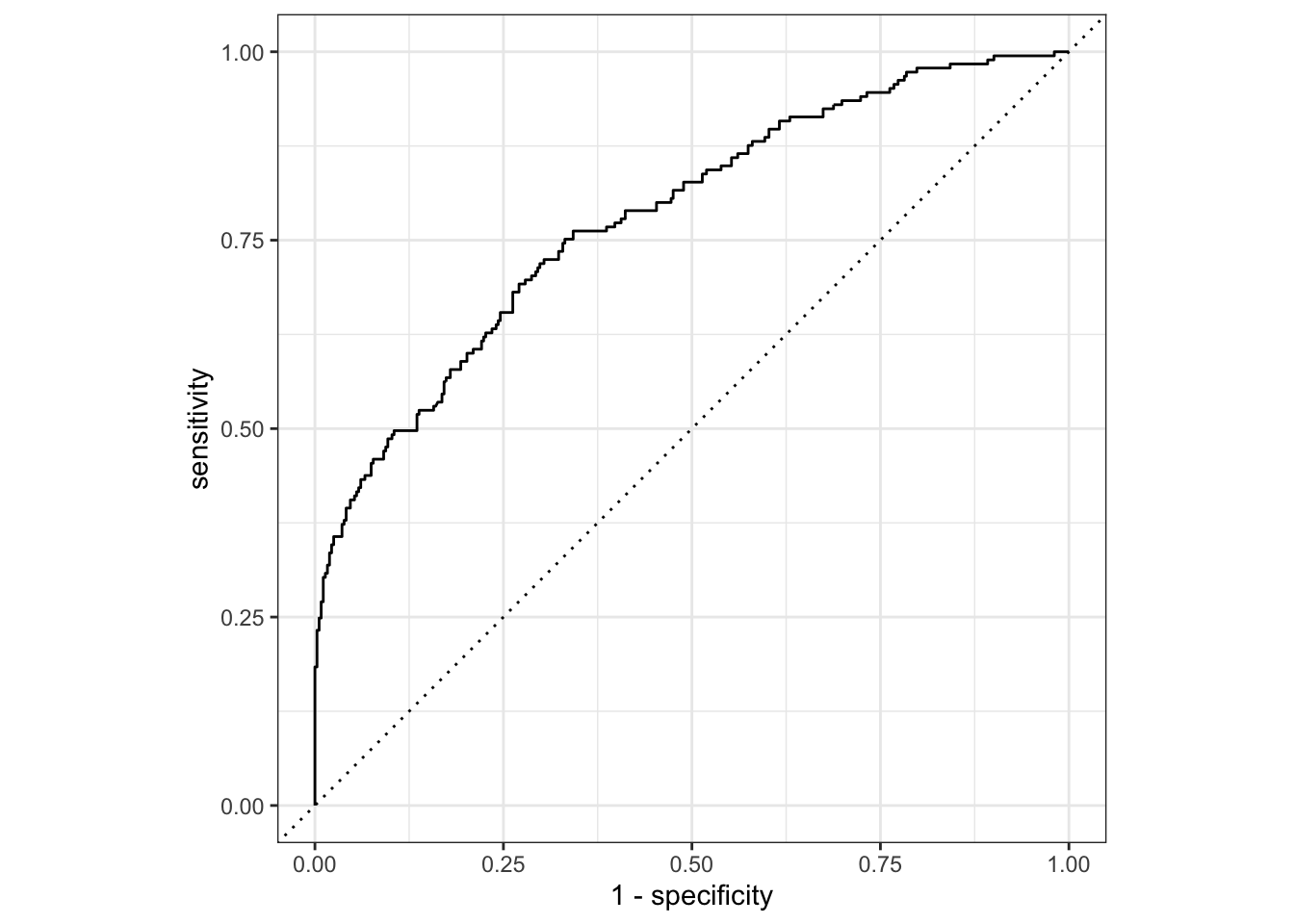
1 roc_auc binary         0.782

ROC-AUC is ok

Model assessment on testing data: ROC curve

set.seed(626)
nausea_fit_test <- nausea_log_wf %>% 
  fit(data = test_data)

nausea_fit_test %>% extract_fit_parsnip() %>% 
  tidy()

# A tibble: 38 × 5
   term                 estimate std.error statistic p.value
   <chr>                   <dbl>     <dbl>     <dbl>   <dbl>
 1 (Intercept)           -10.6      18.7      -0.566 0.571  
 2 SwollenLymphNodesYes   -1.07      0.481    -2.22  0.0263 
 3 ChestCongestionYes      0.779     0.504     1.55  0.122  
 4 ChillsSweatsYes        -0.685     0.608    -1.13  0.260  
 5 NasalCongestionYes      0.592     0.573     1.03  0.301  
 6 CoughYNYes             -0.310     1.05     -0.294 0.769  
 7 SneezeYes               0.478     0.458     1.04  0.297  
 8 FatigueYes              0.223     1.08      0.208 0.835  
 9 SubjectiveFeverYes      1.72      0.556     3.10  0.00195
10 HeadacheYes             0.542     0.688     0.788 0.430  
# … with 28 more rows

nausea_aug_test2 <- augment(nausea_fit_test, test_data)

nausea_aug_test2 %>% 
  roc_curve(truth = Nausea, .pred_Yes, event_level = "second") %>% 
  autoplot()

nausea_aug_test2 %>% roc_auc(truth = Nausea, .pred_Yes, 
                            event_level = "second")

# A tibble: 1 × 3
  .metric .estimator .estimate
  <chr>   <chr>          <dbl>
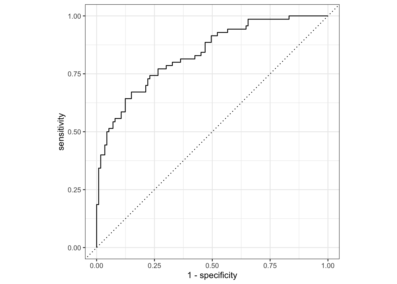
1 roc_auc binary         0.836

The testing data out-performed the training set

Model 2 fitting: runny nose to predict nausea

Create new recipe and workflow

recipe_nausea2 <- recipe(Nausea ~RunnyNose, data = train_data) #only include runny nose

nausea_log_wf2 <- workflow() %>% 
  add_model(log_mod) %>% #model definition, use the same as Model 1
  add_recipe(recipe_nausea2) #model recipe

Model fitting

set.seed(626)
nausea_fit2 <- nausea_log_wf2 %>% 
  fit(data = train_data)

nausea_fit2 %>% extract_fit_parsnip() %>% 
  tidy()

# A tibble: 2 × 5
  term         estimate std.error statistic    p.value
  <chr>           <dbl>     <dbl>     <dbl>      <dbl>
1 (Intercept)   -0.738      0.165    -4.46  0.00000806
2 RunnyNoseYes   0.0961     0.198     0.487 0.626

Model assessment on training data

set.seed(626)
nausea_aug_test2 <- augment(nausea_fit2, train_data)

nausea_aug_test2 %>% 
  roc_curve(truth = Nausea, .pred_Yes, event_level = "second") %>% 
  autoplot()

nausea_aug_test2 %>% roc_auc(truth = Nausea, .pred_Yes, 
                            event_level = "second")

# A tibble: 1 × 3
  .metric .estimator .estimate
  <chr>   <chr>          <dbl>
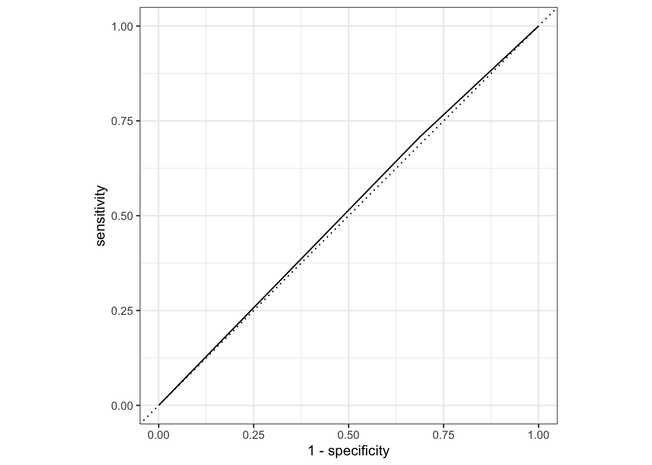
1 roc_auc binary         0.510

The ROC-AUC here is lower than Model 1

Model assessment on testing data

set.seed(626)
nausea_fit_test3 <- nausea_log_wf2 %>% 
  fit(data = test_data)

nausea_fit_test3 %>% extract_fit_parsnip() %>% 
  tidy()

# A tibble: 2 × 5
  term         estimate std.error statistic p.value
  <chr>           <dbl>     <dbl>     <dbl>   <dbl>
1 (Intercept)    -0.368     0.307    -1.20    0.230
2 RunnyNoseYes   -0.147     0.353    -0.416   0.677

nausea_aug_test3 <- augment(nausea_fit_test3, test_data)

nausea_aug_test3 %>% 
  roc_curve(truth = Nausea, .pred_Yes, event_level = "second") %>% 
  autoplot()

nausea_aug_test3 %>% roc_auc(truth = Nausea, .pred_Yes, 
                            event_level = "second")

# A tibble: 1 × 3
  .metric .estimator .estimate
  <chr>   <chr>          <dbl>
1 roc_auc binary         0.514

The testing data is no different. Runny nose is likely not a good predictor of nausea.

This Section added by Nathan Greenslit

Model 3 fitting: all variables to predict Body Temperature

Define the model: linear regression

lin_mod <- linear_reg() %>% #model type is linear regression 
  set_engine("lm") #engine set to  linear model

Create recipe for Multivariate model

recipe_bt_all <- recipe(BodyTemp ~., data = train_data)

Body Temp is the outcome and all other variables are predictors

Create workflow: combine model definition and recipe

bt_lin_wf_all <- workflow() %>% 
  add_model(lin_mod) %>% #model definition 
  add_recipe(recipe_bt_all) #model recipe

This will run a linear regression on the flu data, predicting body temperature using all other variables that we kept.

Multivariate Model Fitting

bt_fit_all <- bt_lin_wf_all %>% 
  fit(data = train_data)

bt_fit_all %>% extract_fit_parsnip() %>% 
  tidy()

# A tibble: 38 × 5
   term                 estimate std.error statistic   p.value
   <chr>                   <dbl>     <dbl>     <dbl>     <dbl>
 1 (Intercept)           97.9        0.354   277.    0        
 2 SwollenLymphNodesYes  -0.204      0.108    -1.89  0.0599   
 3 ChestCongestionYes     0.0863     0.114     0.759 0.448    
 4 ChillsSweatsYes        0.100      0.158     0.637 0.525    
 5 NasalCongestionYes    -0.376      0.134    -2.81  0.00517  
 6 CoughYNYes             0.459      0.291     1.58  0.115    
 7 SneezeYes             -0.470      0.117    -4.02  0.0000658
 8 FatigueYes             0.424      0.181     2.35  0.0191   
 9 SubjectiveFeverYes     0.488      0.125     3.89  0.000112 
10 HeadacheYes            0.0343     0.146     0.235 0.815    
# … with 28 more rows

Model assessment on training data: RMSE and Rsq

set.seed(626)
bt_aug_train_all <- augment(bt_fit_all, train_data) #pull in train data

Warning in predict.lm(object = object$fit, newdata = new_data, type =
"response"): prediction from a rank-deficient fit may be misleading

### RMSE and R2 to test model performance

rmse1 <- bt_aug_train_all %>% rmse(truth = BodyTemp, .pred) #RMSE
rsq1 <- bt_aug_train_all %>% rsq(truth = BodyTemp, .pred) #RSQ
bt_metrics_all_train<- full_join(rmse1, rsq1)

Joining with `by = join_by(.metric, .estimator, .estimate)`

bt_metrics_all_train

# A tibble: 2 × 3
  .metric .estimator .estimate
  <chr>   <chr>          <dbl>
1 rmse    standard       1.12 
2 rsq     standard       0.166

Model assessment on testing data: RMSE and Rsq

set.seed(626)
bt_fit_test_all <- bt_lin_wf_all %>% 
  fit(data = test_data) #pull in test data

bt_fit_test_all %>% extract_fit_parsnip() %>% 
  tidy()

# A tibble: 38 × 5
   term                 estimate std.error statistic   p.value
   <chr>                   <dbl>     <dbl>     <dbl>     <dbl>
 1 (Intercept)           98.7        0.655   151.    6.80e-164
 2 SwollenLymphNodesYes  -0.0195     0.186    -0.105 9.17e-  1
 3 ChestCongestionYes     0.297      0.205     1.45  1.49e-  1
 4 ChillsSweatsYes        0.279      0.233     1.20  2.34e-  1
 5 NasalCongestionYes     0.0556     0.229     0.243 8.09e-  1
 6 CoughYNYes            -0.210      0.427    -0.491 6.24e-  1
 7 SneezeYes             -0.175      0.193    -0.906 3.66e-  1
 8 FatigueYes            -0.527      0.411    -1.28  2.02e-  1
 9 SubjectiveFeverYes     0.266      0.195     1.37  1.74e-  1
10 HeadacheYes            0.128      0.263     0.487 6.27e-  1
# … with 28 more rows

bt_aug_test_all <- augment(bt_fit_test_all, test_data)

Warning in predict.lm(object = object$fit, newdata = new_data, type =
"response"): prediction from a rank-deficient fit may be misleading

### RMSE and R2 to test model performance

rmse2 <- bt_aug_test_all %>% rmse(truth = BodyTemp, .pred) #RMSE
rsq2 <- bt_aug_test_all %>% rsq(truth = BodyTemp, .pred) #RSQ
bt_metrics_all_test<- full_join(rmse2, rsq2)

Joining with `by = join_by(.metric, .estimator, .estimate)`

bt_metrics_all_test

# A tibble: 2 × 3
  .metric .estimator .estimate
  <chr>   <chr>          <dbl>
1 rmse    standard       0.950
2 rsq     standard       0.223

Here it looks like the test data outperformed the model data (lower rmse and higher rsq).

Model 4 fitting: runny nose to predict Body Temperature

Create new recipe and workflow

recipe_bt2 <- recipe(BodyTemp ~RunnyNose, data = train_data) #only include runny nose

bt_lin_wf2 <- workflow() %>% 
  add_model(lin_mod) %>% #model definition, use the same as Model 1
  add_recipe(recipe_bt2) #model recipe

Model fitting

bt_fit2 <- bt_lin_wf2 %>% 
  fit(data = train_data)

bt_fit2 %>% extract_fit_parsnip() %>% 
  tidy()

# A tibble: 2 × 5
  term         estimate std.error statistic p.value
  <chr>           <dbl>     <dbl>     <dbl>   <dbl>
1 (Intercept)    99.2      0.0947   1048.   0      
2 RunnyNoseYes   -0.318    0.114      -2.80 0.00537

Model assessment on training data

set.seed(626)
bt_aug_train_uni <- augment(bt_fit2, train_data) #Train Data

### RMSE and R2 to test model performance

rmse3 <- bt_aug_train_uni %>% rmse(truth = BodyTemp, .pred) #RMSE
rsq3 <- bt_aug_train_uni %>% rsq(truth = BodyTemp, .pred) #RSQ
bt_metrics_uni_train<- full_join(rmse3, rsq3)

Joining with `by = join_by(.metric, .estimator, .estimate)`

bt_metrics_uni_train

# A tibble: 2 × 3
  .metric .estimator .estimate
  <chr>   <chr>          <dbl>
1 rmse    standard      1.22  
2 rsq     standard      0.0141

Model assessment on testing data

set.seed(626)
bt_fit_test_uni <- bt_lin_wf2 %>% 
  fit(data = test_data)

bt_fit_test_uni %>% extract_fit_parsnip() %>% 
  tidy()

# A tibble: 2 × 5
  term         estimate std.error statistic   p.value
  <chr>           <dbl>     <dbl>     <dbl>     <dbl>
1 (Intercept)    99.0       0.163   607.    2.12e-301
2 RunnyNoseYes   -0.172     0.187    -0.918 3.60e-  1

bt_aug_test_uni <- augment(bt_fit_test_uni, test_data) #Test Data

### RMSE and R2 to test model performance

rmse4 <- bt_aug_test_uni %>% rmse(truth = BodyTemp, .pred) #RMSE
rsq4 <- bt_aug_test_uni %>% rsq(truth = BodyTemp, .pred) #RSQ
bt_metrics_uni_test<- full_join(rmse4, rsq4)

Joining with `by = join_by(.metric, .estimator, .estimate)`

bt_metrics_uni_test

# A tibble: 2 × 3
  .metric .estimator .estimate
  <chr>   <chr>          <dbl>
1 rmse    standard     1.08   
2 rsq     standard     0.00464

Here, the training data outperformed the model data, but either way, it does not look like Runny nose is a good predictor of Body Temperature.

Ultimately, our multivariate linear regression provided better performance assessments, so there is more exploring to be done!