library(here)
library(tidyverse)
library(rsample) #Data split
library(tidymodels)
library(rpart) #Model fit
library(ranger) #Model fit
library(glmnet) #Model fit
library(rpart.plot)  #viz of decision tree
library(vip) #viz of variable importance plots
library(ggpmisc) #for adding linear regression to plotsMachine Learning
Load packages
Load data
data <- readRDS(here("fluanalysis/data/processed_data/symptoms_clean.RDS"))Data splitting
set.seed(123)

data_split <- initial_split(
  data, prop = 7/10, #70:30 Split
  strata = BodyTemp) #more balanced outcomes across train/test split

train <- training(data_split)
test  <- testing(data_split)
Create recipes for later use
#Training data
bt_rec_train <- recipe(BodyTemp~., data = train) %>%
  step_dummy(all_nominal(), -all_outcomes()) %>% #pick nominal predictors
  step_ordinalscore() %>%
  step_zv(all_predictors())

#Testing data
bt_rec_test <- recipe(BodyTemp~., data = test) %>%
  step_dummy(all_nominal(), -all_outcomes()) %>% #pick nominal predictors
  step_ordinalscore() %>%
  step_zv(all_predictors())
Null Model
5-Fold Cross Validation
fold_bt_train <- vfold_cv(train, v = 5, repeats = 5, strata = BodyTemp)

fold_bt_test <- vfold_cv(test, v = 5, repeats = 5, strata = BodyTemp)
Create recipe
#Train Data
rec_train <-
  recipe(BodyTemp ~ ., data = train) %>% #predict BodyTemp with all variables
  step_dummy(all_nominal(), -all_outcomes()) %>% #pick nominal predictors
  step_ordinalscore() %>%
  step_zv(all_predictors())

#Test Data
rec_test <-
  recipe(BodyTemp ~ ., data = train) %>%
  step_dummy(all_nominal(), -all_outcomes()) %>%
  step_ordinalscore() %>%
  step_zv(all_predictors())
Define Model
lm_mod <- linear_reg() %>%
  set_engine("lm") %>%
  set_mode("regression")
Create workflows
#training data
null_train_wf <- workflow() %>%
  add_model(lm_mod) %>%
  add_recipe(bt_rec_train)

#testing data
null_test_wf <- workflow() %>%
  add_model(lm_mod) %>%
  add_recipe(bt_rec_test)
Fit models
#training data
null_train_fit <- fit_resamples(null_train_wf, resamples = fold_bt_train)

null_test_fit <- fit_resamples(null_test_wf, resamples = fold_bt_test)
Compare train/test metrics
null_train_met <- collect_metrics(null_train_fit)
null_train_met
# A tibble: 2 × 6
.metric .estimator mean n std_err .config
<chr> <chr> <dbl> <int> <dbl> <chr>
1 rmse standard 1.17 25 0.0171 Preprocessor1_Model1
2 rsq standard 0.0849 25 0.00815 Preprocessor1_Model1null_test_met <- collect_metrics(null_test_fit)
null_test_met# A tibble: 2 × 6
.metric .estimator mean n std_err .config
<chr> <chr> <dbl> <int> <dbl> <chr>
1 rmse standard 1.27 25 0.0273 Preprocessor1_Model1
2 rsq standard 0.0146 25 0.00444 Preprocessor1_Model1Training RMSE: 1.21
Testing RMSE: 1.16
Tree model tuning and fitting
Specify model
tune_spec_dtree <- decision_tree(
    cost_complexity = tune(),
    tree_depth = tune()) %>%
  set_engine("rpart") %>%
  set_mode("regression")

tune_spec_dtree
Decision Tree Model Specification (regression)
Main Arguments:
cost_complexity = tune()
tree_depth = tune()
Computational engine: rpart Create workflow
dtree_wf <- workflow() %>%
  add_model(tune_spec_dtree) %>%
  add_recipe(bt_rec_train)
Create grid for model tuning
tree_grid_dtree <-
  grid_regular(
    cost_complexity(),
    tree_depth(),
    levels = 5)

tree_grid_dtree
# A tibble: 25 × 2
cost_complexity tree_depth
<dbl> <int>
1 0.0000000001 1
2 0.0000000178 1
3 0.00000316 1
4 0.000562 1
5 0.1 1
6 0.0000000001 4
7 0.0000000178 4
8 0.00000316 4
9 0.000562 4
10 0.1 4
# … with 15 more rowsUse cross-validation for tuning
dtree_resample <- dtree_wf %>%
  tune_grid(
    resamples = fold_bt_train,
    grid = tree_grid_dtree)
dtree_resample %>%
collect_metrics()# A tibble: 50 × 8
cost_complexity tree_depth .metric .estimator mean n std_err .config
<dbl> <int> <chr> <chr> <dbl> <int> <dbl> <chr>
1 0.0000000001 1 rmse standard 1.19 25 0.0170 Prepro…
2 0.0000000001 1 rsq standard 0.0383 25 0.00415 Prepro…
3 0.0000000178 1 rmse standard 1.19 25 0.0170 Prepro…
4 0.0000000178 1 rsq standard 0.0383 25 0.00415 Prepro…
5 0.00000316 1 rmse standard 1.19 25 0.0170 Prepro…
6 0.00000316 1 rsq standard 0.0383 25 0.00415 Prepro…
7 0.000562 1 rmse standard 1.19 25 0.0170 Prepro…
8 0.000562 1 rsq standard 0.0383 25 0.00415 Prepro…
9 0.1 1 rmse standard 1.21 25 0.0169 Prepro…
10 0.1 1 rsq standard NaN 0 NA Prepro…
# … with 40 more rowsModel plotting
dtree_resample %>% collect_metrics() %>%
mutate(tree_depth = factor(tree_depth)) %>%
ggplot(aes(cost_complexity, mean, color = tree_depth)) +
geom_line(linewidth = 1.5, alpha = 0.6) +
geom_point(size = 2) +
facet_wrap(~ .metric, scales = "free", nrow = 2) +
scale_x_log10(labels = scales::label_number()) +
scale_color_viridis_d(option = "plasma", begin = .9, end = 0)Warning: Removed 5 rows containing missing values (`geom_line()`).Warning: Removed 5 rows containing missing values (`geom_point()`).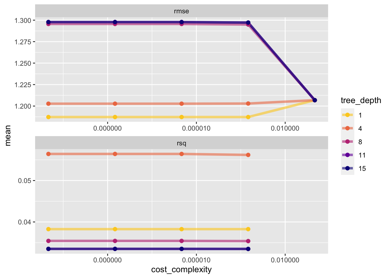
Select the best model
The show_best() function shows us the top 5 candidate models by default. We set n=1
dtree_resample %>%
  show_best(n=1)
Warning: No value of `metric` was given; metric 'rmse' will be used.# A tibble: 1 × 8
cost_complexity tree_depth .metric .estimator mean n std_err .config
<dbl> <int> <chr> <chr> <dbl> <int> <dbl> <chr>
1 0.0000000001 1 rmse standard 1.19 25 0.0170 Preprocesso…Tree model RMSE: 1.23
Tree depth of 1 has the best performance metrics
#Selects best performing model
best_tree <- dtree_resample %>%
  select_best() #pull out best performing hyperparameters

best_tree
# A tibble: 1 × 3
cost_complexity tree_depth .config
<dbl> <int> <chr>
1 0.0000000001 1 Preprocessor1_Model01Create final fit based on best model
Update workflow
dtree_final_wf <- dtree_wf %>%
  finalize_workflow(best_tree) #update workflow with values from select_best()

dtree_final_wf
══ Workflow ════════════════════════════════════════════════════════════════════
Preprocessor: Recipe
Model: decision_tree()
── Preprocessor ────────────────────────────────────────────────────────────────
3 Recipe Steps
• step_dummy()
• step_ordinalscore()
• step_zv()
── Model ───────────────────────────────────────────────────────────────────────
Decision Tree Model Specification (regression)
Main Arguments:
cost_complexity = 1e-10
tree_depth = 1
Computational engine: rpart Fit model to training data
dtree_final_fit <- dtree_final_wf %>%
  fit(train)
Evaluate final fit
Calculating residuals
dtree_residuals <- dtree_final_fit %>%
  augment(train) %>% #use augment() to make predictions
  select(c(.pred, BodyTemp)) %>%
  mutate(.resid = BodyTemp - .pred) #calculate residuals

dtree_residuals
# A tibble: 508 × 3
.pred BodyTemp .resid
<dbl> <dbl> <dbl>
1 99.2 97.8 -1.44
2 99.2 98.1 -1.14
3 98.7 98.1 -0.591
4 98.7 98.2 -0.491
5 98.7 97.8 -0.891
6 98.7 98.2 -0.491
7 98.7 98.1 -0.591
8 99.2 98 -1.24
9 99.2 97.7 -1.54
10 99.2 98.2 -1.04
# … with 498 more rowsPlot predictions vs. true value
dtree_pred_plot <- ggplot(dtree_residuals,
                          aes(x = BodyTemp,
                              y = .pred)) +
  geom_point() +
  labs(title = "Predictions vs Actual: Decision Tree",
       x = "Body Temperature Outcome",
       y = "Body Temperature Prediction")
dtree_pred_plot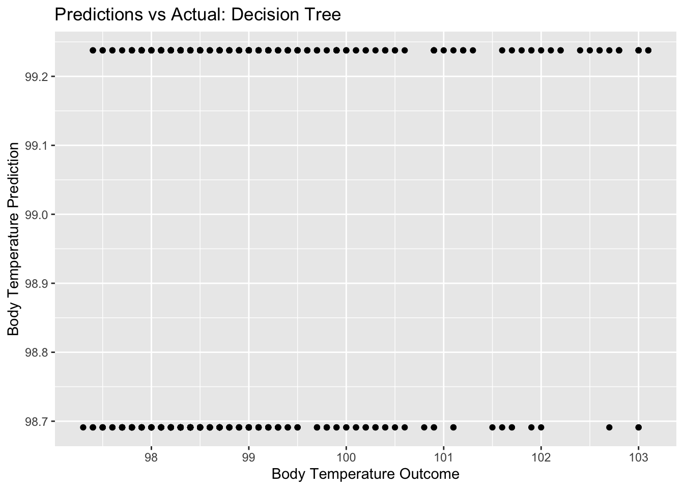
Plot residuals vs. predictions
dtree_residual_plot <- ggplot(dtree_residuals,
                              aes(y = .resid,
                                  x = .pred)) +
  geom_point() +
  labs(title = "Predictions vs Residuals: Decision Tree",
       x = "Body Temperature Prediction",
       y = "Residuals")
plot(dtree_residual_plot) #view plot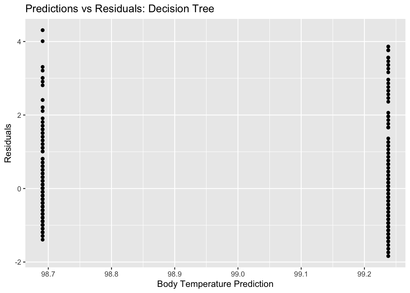
LASSO model tuning and fitting
Specify Model
lasso_mod <- linear_reg(penalty = tune(), mixture = 1) %>%
  set_engine("glmnet")
Setting mixture to a value of one means that the glmnet model will potentially remove irrelevant predictors and choose a simpler model.
Create Workflow
lasso_wf <- workflow() %>%
  add_model(lasso_mod) %>%
  add_recipe(bt_rec_train)
Creating a Tuning Grid
lasso_grid <- tibble(penalty = 10^seq(-3, 0, length.out = 30))Use cross-validation for tuning
lasso_resample <- lasso_wf %>%
  tune_grid(resamples = fold_bt_train,
            grid = lasso_grid,
            control = control_grid(verbose = FALSE, save_pred = TRUE),
            metrics = metric_set(rmse))

lasso_resample %>%
  collect_metrics()
# A tibble: 30 × 7
penalty .metric .estimator mean n std_err .config
<dbl> <chr> <chr> <dbl> <int> <dbl> <chr>
1 0.001 rmse standard 1.17 25 0.0170 Preprocessor1_Model01
2 0.00127 rmse standard 1.17 25 0.0170 Preprocessor1_Model02
3 0.00161 rmse standard 1.17 25 0.0170 Preprocessor1_Model03
4 0.00204 rmse standard 1.17 25 0.0170 Preprocessor1_Model04
5 0.00259 rmse standard 1.17 25 0.0170 Preprocessor1_Model05
6 0.00329 rmse standard 1.17 25 0.0169 Preprocessor1_Model06
7 0.00418 rmse standard 1.17 25 0.0169 Preprocessor1_Model07
8 0.00530 rmse standard 1.17 25 0.0168 Preprocessor1_Model08
9 0.00672 rmse standard 1.16 25 0.0168 Preprocessor1_Model09
10 0.00853 rmse standard 1.16 25 0.0167 Preprocessor1_Model10
# … with 20 more rowsModel plotting
lr_plot <- lasso_resample %>%
  collect_metrics() %>%
  ggplot(aes(x = penalty, y = mean)) +
  geom_point() +
  geom_line() +
  scale_x_log10(labels = scales::label_number())

lr_plot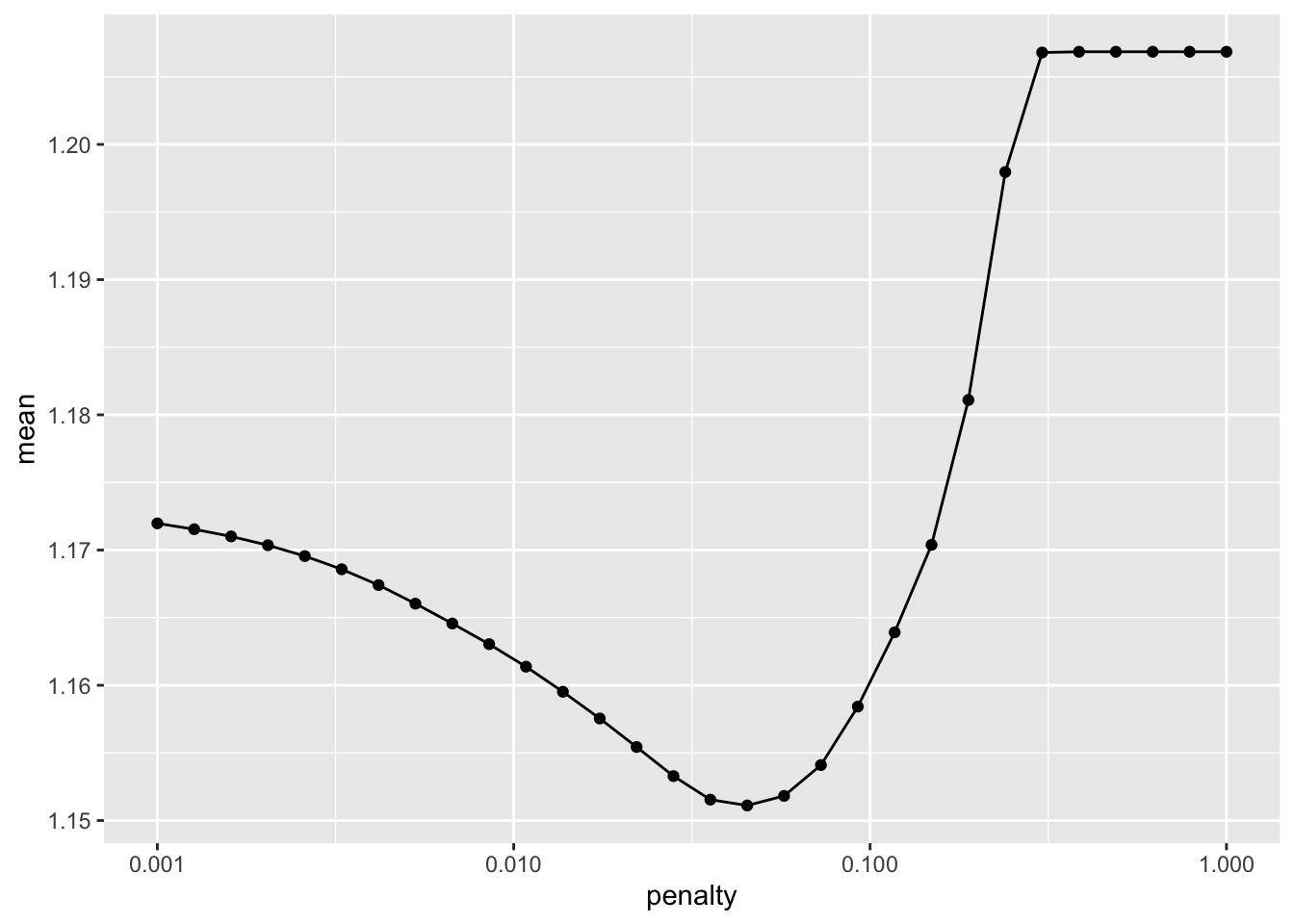
Select the best model
#Show best model
lasso_resample %>% show_best(n=1)
# A tibble: 1 × 7
penalty .metric .estimator mean n std_err .config
<dbl> <chr> <chr> <dbl> <int> <dbl> <chr>
1 0.0452 rmse standard 1.15 25 0.0162 Preprocessor1_Model17#Select best model
best_lasso <- lasso_resample %>%
select_best()Lasso model RMSE: 1.18 (slightly better than Tree)
Create final fit based on best model
lasso_final_wf <- lasso_wf %>%
  finalize_workflow(best_lasso) #update workflow with best model

lasso_final_fit <- lasso_final_wf %>%
  fit(train) #fit updated workflow to training data
Evaluate final fit
Calculating residuals
lasso_residuals <- lasso_final_fit %>%
  augment(train) %>% #use augment() to make predictions from train data
  select(c(.pred, BodyTemp)) %>%
  mutate(.resid = BodyTemp - .pred) #calculate residuals and make new row.

lasso_residuals
# A tibble: 508 × 3
.pred BodyTemp .resid
<dbl> <dbl> <dbl>
1 98.7 97.8 -0.913
2 98.8 98.1 -0.705
3 98.5 98.1 -0.391
4 98.8 98.2 -0.637
5 98.7 97.8 -0.947
6 98.6 98.2 -0.401
7 98.2 98.1 -0.147
8 99.3 98 -1.28
9 98.8 97.7 -1.11
10 99.0 98.2 -0.790
# … with 498 more rowsPlot predictions vs. true value
lasso_pred_plot <- ggplot(lasso_residuals,
                          aes(x = BodyTemp,
                              y = .pred)) +
  geom_point() +
  labs(title = "Predictions vs Actual: LASSO",
       x = "Body Temperature Outcome",
       y = "Body Temperature Prediction") +
  stat_poly_line() +
  stat_poly_eq()
lasso_pred_plot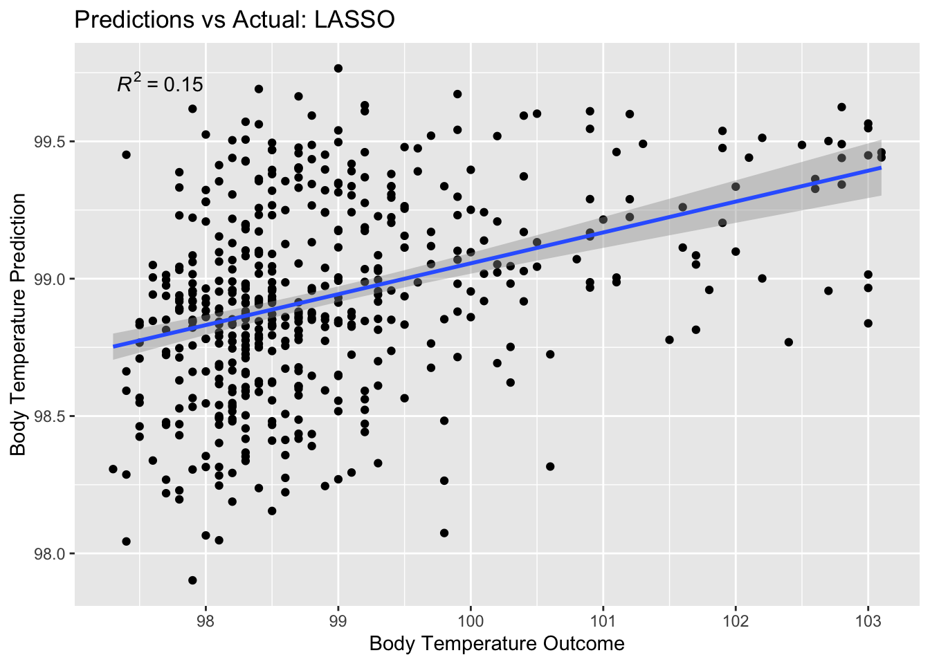
RSQ is low but there is still a positive correlation there (which is good)
Plot residuals vs. predictions
lasso_residual_plot <- ggplot(lasso_residuals,
                              aes(y = .resid,
                                  x = .pred)) +
  geom_point() +
  labs(title = "Predictions vs Residuals: LASSO",
       x = "Body Temperature Prediction",
       y = "Residuals") +
   stat_poly_line() +
  stat_poly_eq()
plot(lasso_residual_plot) #view plot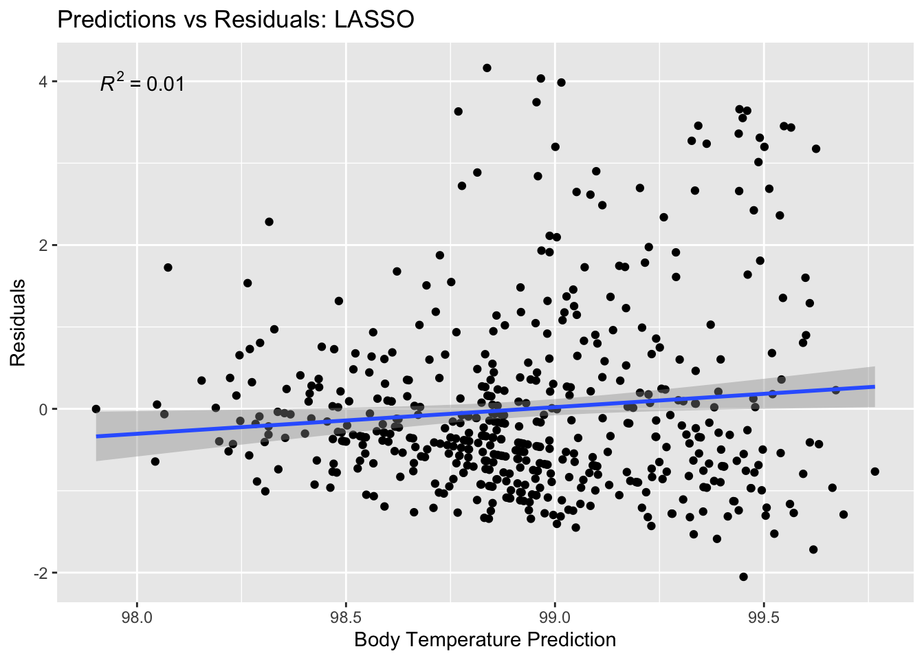
There should be no relationship here, which there isn’t.
Random Forest model tuning and fitting
Detect cores for RFM computation
cores <- parallel::detectCores()
cores
[1] 4Specify Model
rf_mod <- rand_forest(mtry = tune(), min_n = tune(), trees = 1000) %>%
  set_engine("ranger", num.threads = cores) %>%
  set_mode("regression")
Create workflow
rf_wf <- workflow() %>% add_model(rf_mod) %>%
  add_recipe(bt_rec_train)
Create grid for model tuning
rf_grid  <- expand.grid(mtry = c(3, 4, 5, 6),
                        min_n = c(40,50,60),
                        trees = c(500,1000))
Use cross-validation for tuning
rf_resample <- rf_wf %>%
  tune_grid(fold_bt_train,
            grid = 25,
            control = control_grid(save_pred = TRUE),
            metrics = metric_set(rmse))
Check CV metrics
rf_resample %>%
  collect_metrics()
# A tibble: 25 × 8
mtry min_n .metric .estimator mean n std_err .config
<int> <int> <chr> <chr> <dbl> <int> <dbl> <chr>
1 8 38 rmse standard 1.16 25 0.0160 Preprocessor1_Model01
2 29 14 rmse standard 1.20 25 0.0162 Preprocessor1_Model02
3 24 2 rmse standard 1.22 25 0.0158 Preprocessor1_Model03
4 15 31 rmse standard 1.17 25 0.0160 Preprocessor1_Model04
5 7 32 rmse standard 1.16 25 0.0164 Preprocessor1_Model05
6 20 9 rmse standard 1.20 25 0.0159 Preprocessor1_Model06
7 13 7 rmse standard 1.19 25 0.0163 Preprocessor1_Model07
8 2 15 rmse standard 1.17 25 0.0164 Preprocessor1_Model08
9 23 28 rmse standard 1.18 25 0.0161 Preprocessor1_Model09
10 23 4 rmse standard 1.22 25 0.0158 Preprocessor1_Model10
# … with 15 more rowsModel performance plotting
rf_resample %>% autoplot()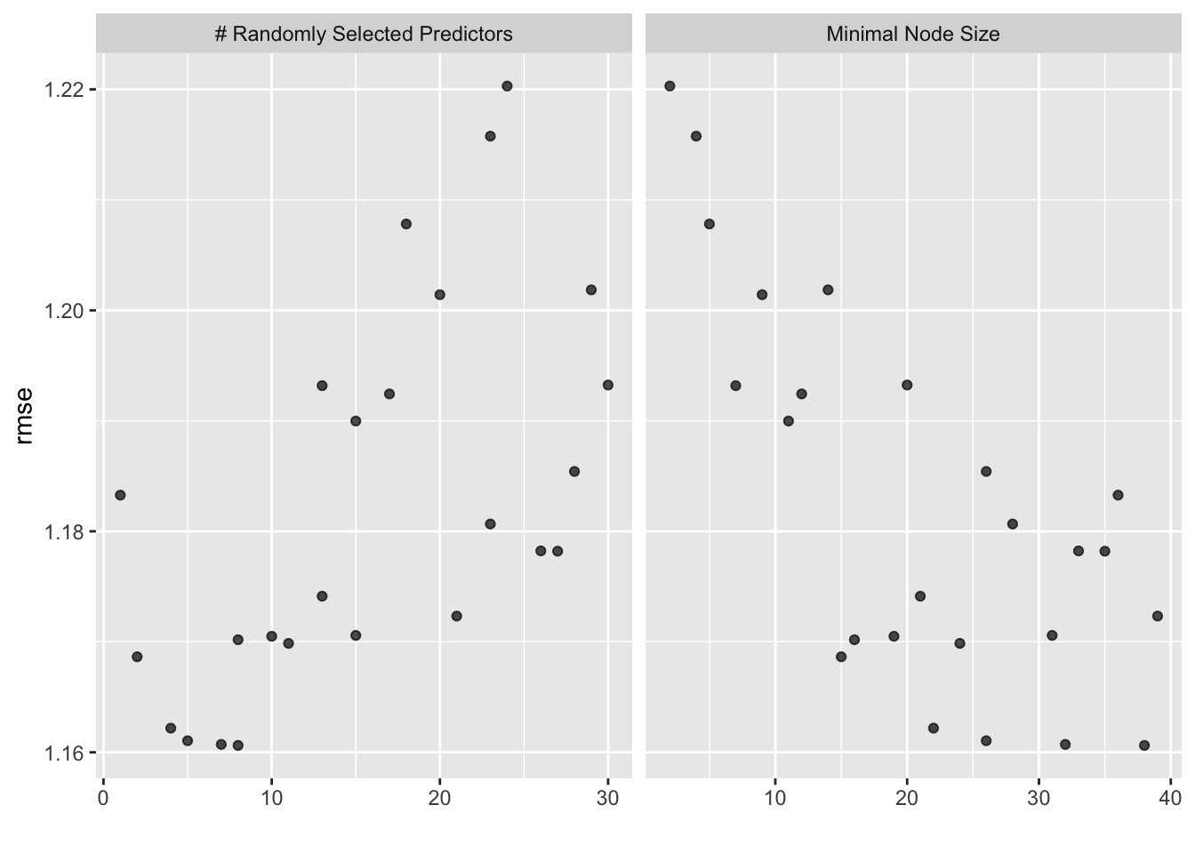
Select the best model
#Show best model
rf_resample %>%
  show_best(n=1)
# A tibble: 1 × 8
mtry min_n .metric .estimator mean n std_err .config
<int> <int> <chr> <chr> <dbl> <int> <dbl> <chr>
1 8 38 rmse standard 1.16 25 0.0160 Preprocessor1_Model01#Select best model
best_rf <- rf_resample %>%
select_best(method = "rmse")Random forest model RMSE: 1.20
Create final fit based on best model
rf_final_wf <-
  rf_wf %>%
  finalize_workflow(best_rf) #update workflow with best model

rf_final_fit <-
  rf_final_wf %>%
  fit(train) #fit best model to training data
Evaluate final fit
Calculating residuals
rf_residuals <- rf_final_fit %>%
  augment(train) %>% #use augment() to make predictions from train data
  select(c(.pred, BodyTemp)) %>%
  mutate(.resid = BodyTemp - .pred) #calculate residuals and make new row.

rf_residuals
# A tibble: 508 × 3
.pred BodyTemp .resid
<dbl> <dbl> <dbl>
1 98.7 97.8 -0.854
2 98.6 98.1 -0.513
3 98.7 98.1 -0.643
4 98.7 98.2 -0.535
5 98.8 97.8 -1.02
6 98.5 98.2 -0.336
7 98.3 98.1 -0.218
8 99.1 98 -1.12
9 98.8 97.7 -1.07
10 98.8 98.2 -0.644
# … with 498 more rowsPlot predictions vs. true value
rf_pred_plot <- ggplot(rf_residuals,
                          aes(x = BodyTemp,
                              y = .pred)) +
  geom_point() +
  labs(title = "Predictions vs Actual: Random Forest",
       x = "Body Temperature Actual",
       y = "Body Temperature Prediction") +
   stat_poly_line() +
  stat_poly_eq()
rf_pred_plot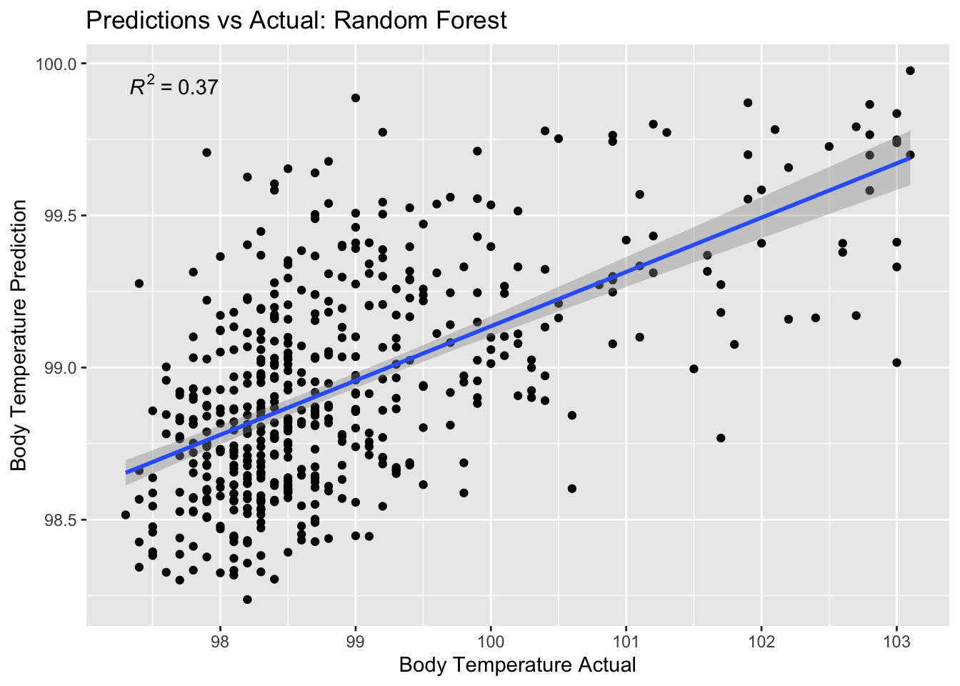
There is a stronger correlation here than in the LASSO or Tree Model
Plot residuals vs. predictions
rf_residual_plot <- ggplot(rf_residuals,
                              aes(y = .resid,
                                  x = .pred)) +
  geom_point() +
  labs(title = "Predictions vs Residuals: Random Forest",
       x = "Body Temperature Prediction",
       y = "Residuals") +
   stat_poly_line() +
  stat_poly_eq()
plot(rf_residual_plot) #view plot
There is a slight correlation here, which is not ideal.
Model Selection
| Model | RMSE | Std_Err |
|---|---|---|
| Null Train | 1.21 | 0.018 |
| Null Test | 1.16 | 0.029 |
| Tree | 1.23 | 0.016 |
| LASSO | 1.18 | 0.017 |
| Random Forest | 1.20 | 0.017 |
Of the three machine learning models we generated, LASSO had the lowest RMSE, but they were all close. The disadvantage with LASSO though is there is a weak correlation between actual value and prediction. However, the advantage of this model is there is no correlation between predictions and residuals.
The Random Forest model also performed decently with the next lowest RMSE. The disadvantage with this model is that there is a slight correlation between predictions and residuals (as prediction value increases, so does the residual), but the advantage is that there is a stronger correlation between actual values and predictions than in the LASSO model.
The Tree model performed the poorest, being the only one that did not out-perform the null model. The plots generated for this model also did not look promising.
I have decided on the Random Forest model as the final model.
Final Evaluation
Once you picked your final model, you are allowed to once – and only once – fit it to the test data and check how well it performs on that data. You can do that using the last_fit() function applied to the model you end up choosing. For the final model applied to the test set, report performance and the diagnostic plots as above.
rf_last_fit <- rf_final_wf %>%
  last_fit(data_split)

rf_last_fit %>% collect_metrics()
# A tibble: 2 × 4
.metric .estimator .estimate .config
<chr> <chr> <dbl> <chr>
1 rmse standard 1.18 Preprocessor1_Model1
2 rsq standard 0.00941 Preprocessor1_Model1RMSE of 1.10 and standard error of 0.012.
This performance is slightly better than the null model.